Dask 101

Context¶

We will be using Dask with Xarray to parallelize our data analysis. The analysis is very similar to what we have done in previous examples but this time we will use data on a global coverage that we read from the SeasFire Cube.

We will learn how to use the EDC Pangeo Dask Gateway to analyse data at scale.

Data¶

In this workshop, we will be using the SeasFire Data Cube published to the EarthCODE Open Science Catalog

Alonso, Lazaro, Gans, Fabian, Karasante, Ilektra, Ahuja, Akanksha, Prapas, Ioannis, Kondylatos, Spyros, Papoutsis, Ioannis, Panagiotou, Eleannna, Michail, Dimitrios, Cremer, Felix, Weber, Ulrich, & Carvalhais, Nuno. (2022). SeasFire Cube: A Global Dataset for Seasonal Fire Modeling in the Earth System (0.4) [Data set]. Zenodo. Alonso et al. (2024). The same dataset can also be downloaded from Zenodo: https://zenodo.org/records/13834057

import dask.distributed
import xarray

Parallelize with Dask¶

We know from previous chapter cloud native formats 101 that chunking is key for analyzing large datasets. In this episode, we will learn to parallelize our data analysis using Dask on our chunked dataset.

What is Dask ?¶

Dask scales the existing Python ecosystem: with very or no changes in your code, you can speed-up computation using Dask or process bigger than memory datasets.

Dask is a flexible library for parallel computing in Python.
It is widely used for handling large and complex Earth Science datasets and speed up science.
Dask is powerful, scalable and flexible. It is the leading platform today for data analytics at scale.
It scales natively to clusters, cloud, HPC and bridges prototyping up to production.
The strength of Dask is that is scales and accelerates the existing Python ecosystem e.g. Numpy, Pandas and Scikit-learn with few effort from end-users.

It is interesting to note that at first, Dask has been created to handle data that is larger than memory, on a single computer. It then was extended with Distributed to compute data in parallel over clusters of computers.

How does Dask scale and accelerate your data analysis?¶

Dask proposes different abstractions to distribute your computation. In this Dask Introduction section, we will focus on Dask Array which is widely used in pangeo ecosystem as a back end of Xarray.

As shown in the previous section Dask Array is based on chunks. Chunks of a Dask Array are well-known Numpy arrays. By transforming our big datasets to Dask Array, making use of chunk, a large array is handled as many smaller Numpy ones and we can compute each of these chunks independently.

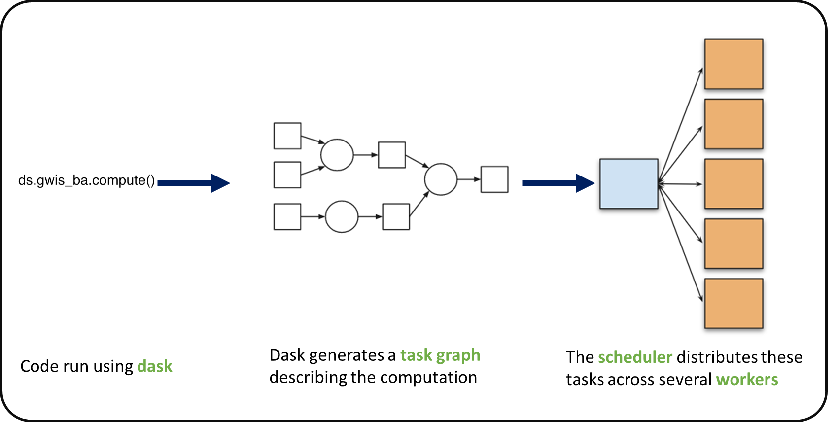
How does Xarray with Dask distribute data analysis?¶

When we use chunks with Xarray, the real computation is only done when needed or asked for, usually when invoking compute() or load() functions. Dask generates a task graph describing the computations to be done. When using Dask Distributed a Scheduler distributes these tasks across several Workers.

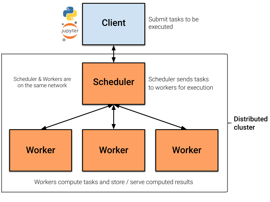
What is a Dask Distributed cluster ?¶

A Dask Distributed cluster is made of two main components:

a Scheduler, responsible for handling computations graph and distributing tasks to Workers.
One or several (up to 1000s) Workers, computing individual tasks and storing results and data into distributed memory (RAM and/or worker’s local disk).

A user usually needs Client and Cluster objects as shown below to use Dask Distributed.

Where can we deploy a Dask distributed cluster?¶

Dask distributed clusters can be deployed on your laptop or on distributed infrastructures (Cloud, HPC centers, Hadoop, etc.) Dask distributed Cluster object is responsible of deploying and scaling a Dask Cluster on the underlying resources.

EDC has one such deployment

Dask distributed Client¶

The Dask distributed Client is what allows you to interact with Dask distributed Clusters. When using Dask distributed, you always need to create a Client object. Once a Client has been created, it will be used by default by each call to a Dask API, even if you do not explicitly use it.

No matter the Dask API (e.g. Arrays, Dataframes, Delayed, Futures, etc.) that you use, under the hood, Dask will create a Directed Acyclic Graph (DAG) of tasks by analysing the code. Client will be responsible to submit this DAG to the Scheduler along with the final result you want to compute. The Client will also gather results from the Workers, and aggregate it back in its underlying Python process.

Using Client() function with no argument, you will create a local Dask cluster with a number of workers and threads per worker corresponding to the number of cores in the ‘local’ machine. Here, during the workshop, we are running this notebook in the EDC Pangeo cloud deployment, so the ‘local’ machine is the jupyterlab you are using at the Cloud, and the number of cores is the number of cores on the cloud computing resources you’ve been given (not on your laptop).

from dask.distributed import Client

client = Client()   # create a local dask cluster on the local machine.
client

Inspecting the Cluster Info section above gives us information about the created cluster: we have 2 or 4 workers and the same number of threads (e.g. 1 thread per worker).

# close client to clean resources
# Note, you can run this tutorial locally if you uncomment this line 
client.close()

Scaling your Computation using Dask Gateway.¶

For this workshop, you will learn how to use Dask Gateway to manage Dask clusters over Kubernetes, allowing to run our data analysis in parallel e.g. distribute tasks across several workers.

Dask Gateway is a component that helps you manage and create Dask Clusters across your environment. As Dask Gateway is configured by default on this infrastructure, you just need to execute the following cells.

Note that, if you’re executing this locally, without prior setup for dask gateway, the following code will crash. If you would like to run this locally, skip these lines and continue with the local dask client above

from dask_gateway import Gateway
gateway = Gateway()

EDC Dask Gateway Options¶

EDC Pangeo’s Dask Gateway provides several cluster configurations for your workloads. You can choose the appropriate size based on your computational needs:

small
- Worker cores: 0.5
- Worker memory: 1 GB
medium
- Worker cores: 2
- Worker memory: 2 GB
larger
- Worker cores: 4
- Worker memory: 4 GB

You can set these options when spawning your Dask clusters to ensure optimal resource allocation.

cluster_options = gateway.cluster_options()
cluster_options

cluster = gateway.new_cluster(cluster_options=cluster_options)
cluster.scale(2)
cluster

Get a client from the Dask Gateway Cluster¶

As stated above, creating a Dask Client is mandatory in order to perform following Daks computations on your Dask Cluster.

client = cluster.get_client()
client

Dask Dashboard¶

Dask comes with a really handy interface: the Dask Dashboard. It is a web interface that you can open in a separated tab of your browser.

We will learn here how to use it through dask jupyterlab extension.

To use Dask Dashboard through jupyterlab extension on Pangeo EDC infrastructure, you will just need too look at the html link you have for your jupyterlab, and Dask dashboard port number, as highlighted in the figure below.

Dash Board link Dash lab

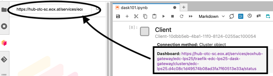
Then click the orange icon indicated in the above figure, and type ‘your’ dashboard link.

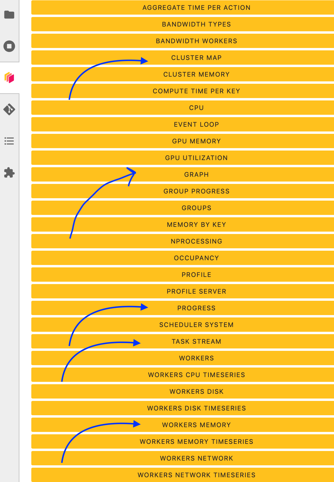
You can click several buttons indicated with blue arrows in above figures, then drag and drop to place them as your convenience.

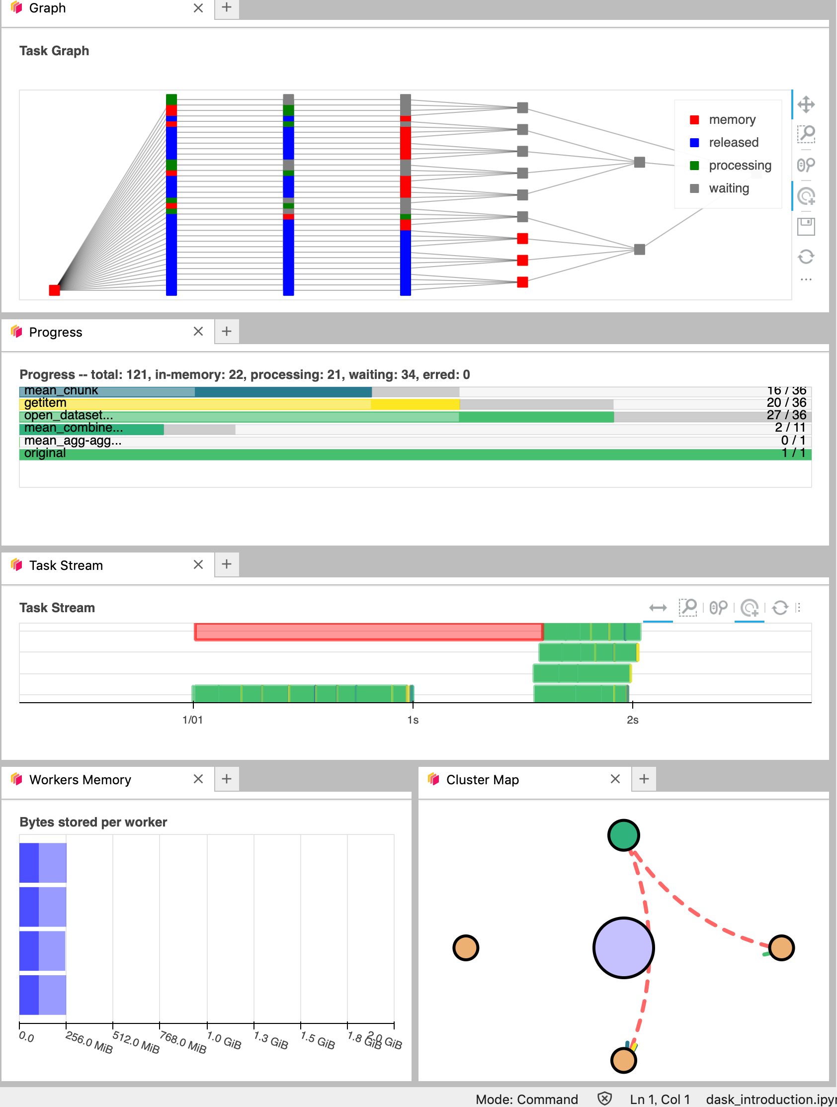
It’s really helpfull to understand your computation and how it is distributed.

Dask Distributed computations on our dataset¶

Let’s open the SeasFire dataset we previously looked at, select a single location over time, visualize the task graph generated by Dask, and observe the Dask Dashboard.

http_url = "https://s3.waw4-1.cloudferro.com/EarthCODE/OSCAssets/seasfire/seasfire_v0.4.zarr/"

ds = xarray.open_dataset(
	http_url,
	engine='zarr',
    chunks={},
	consolidated=True
)
ds

mask= ds['lsm'][:,:]
gwis_all= ds.gwis_ba.resample(time="1YE").sum()
gwis_all= gwis_all.where(mask>0.5)

gwis_2020= gwis_all.sel(time='2020-08-01', method='nearest')
gwis_2020.data

gwis_2020.data.visualize(optimize_graph=True)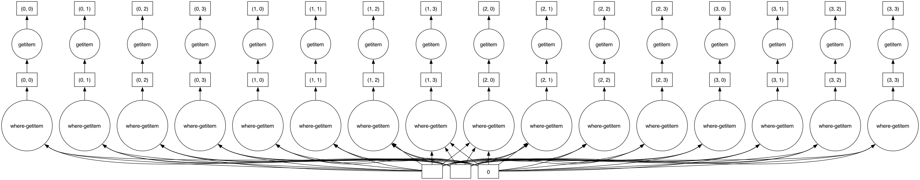

Did you notice something on the Dask Dashboard when running the two previous cells?

We didn’t ‘compute’ anything. We just built a Dask task graph with it’s size indicated as count above, but did not ask Dask to return a result.

Note that underneath, dask optimizes the execution graph (opaquely), so as to minimize overheads and overall execution resources (hence why we’re passing optimize_graph=True)

Computing¶

Calling compute on our Xarray object will trigger the execution on the Dask Cluster. Alternatively any action that would demand the computation of our data (e.g. plotting) would trigger the execution of our workflow.

You should be able to see how Dask is working on Dask Dashboard.

gwis_2020.plot()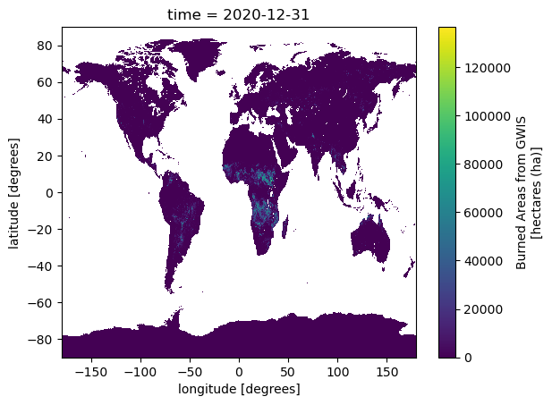

Closing Clusters¶

Close Clusters to Clean Resources for the next exercise (generally a good practice!)

# close client to clean resources
client.close()

References¶

Alonso, L., Gans, F., Karasante, I., Ahuja, A., Prapas, I., Kondylatos, S., Papoutsis, I., Panagiotou, E., Mihail, D., Cremer, F., Weber, U., & Carvalhais, N. (2024). SeasFire Cube: A Global Dataset for Seasonal Fire Modeling in the Earth System. Zenodo. 10.5281/ZENODO.13834057

Welcome

Cloud Native Formats 101